Shading Using Patterns in VCS
This notebook shows how to use patterns in vcs.
Pattern can be used with isofill, boxfill, meshfill and fillarea object.
In this notebook we are using primirarly boxfill
Contents
Prepare Notebook Elements
[1]:
import requests
import cdms2

r = requests.get("https://uvcdat.llnl.gov/cdat/sample_data/clt.nc",stream=True)
with open("clt.nc","wb") as f:
    for chunk in r.iter_content(chunk_size=1024):
        if chunk:  # filter local_filename keep-alive new chunks
            f.write(chunk)

# and load data
f = cdms2.open("clt.nc")
clt = f("clt",time=slice(0,1),squeeze=1) # Get first month
Create default Graphic Method
[2]:
import vcs
import cdms2
x=vcs.init(bg=True)
gm = vcs.createboxfill()
gm.boxfill_type = "custom"
[3]:
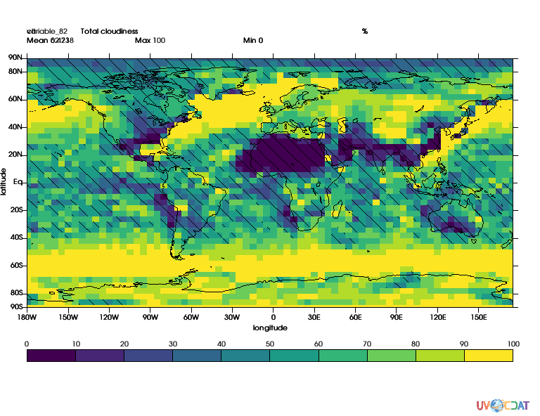
# Let's look at the data w/o pattern
x.plot(clt,gm)
[3]:

Mask some data
Now let’s assume we are only interested in areas where clt is greater than 60% let’s shade out areas where clt is < 60%
[4]:
import MV2
bad = MV2.less(clt,60.).astype("f")
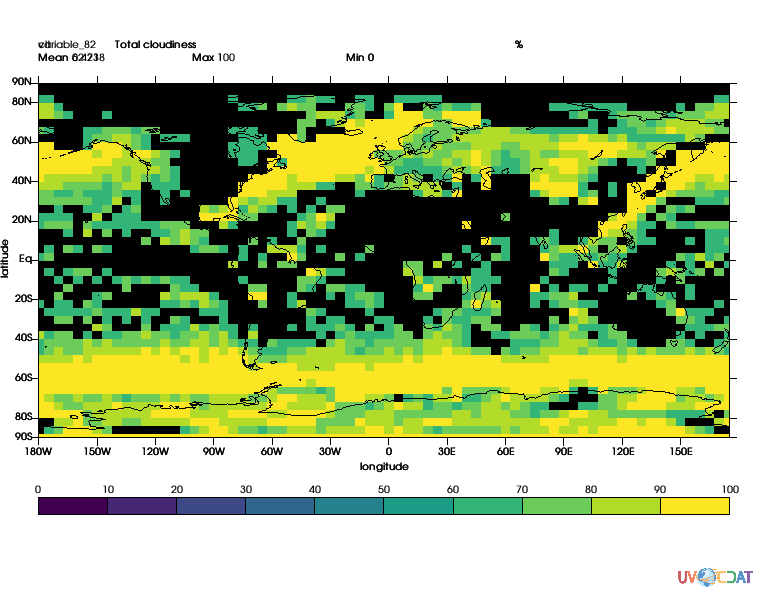
Method 1: Regular Masking
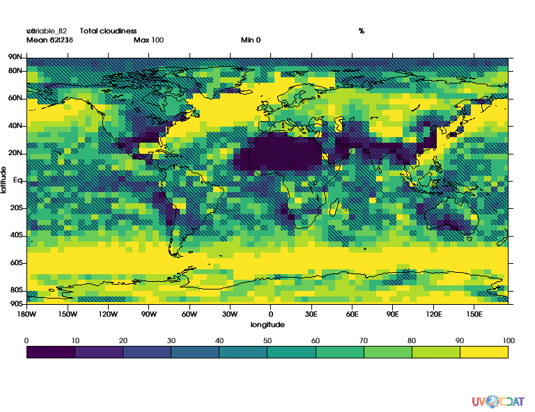
[5]:
# let's create a second boxfill method
gm2 = vcs.createboxfill()
gm2.boxfill_type = "custom"
# and a template for it
tmpl2 = vcs.createtemplate()
tmpl2.legend.priority=0
gm2.levels = [[0.5,1.]]
gm2.fillareacolors = ["black",]
x.plot(bad,gm2,tmpl2)
[5]:
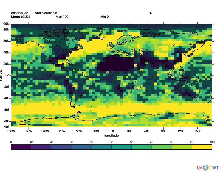
Method 2: Using Opacity
Let’s use some opacity to “see” what’s bellow (top)
[6]:
gm2.fillareaopacity = [50]
x.clear()
x.plot(clt,gm)
x.plot(bad,gm2,tmpl2)
[6]:
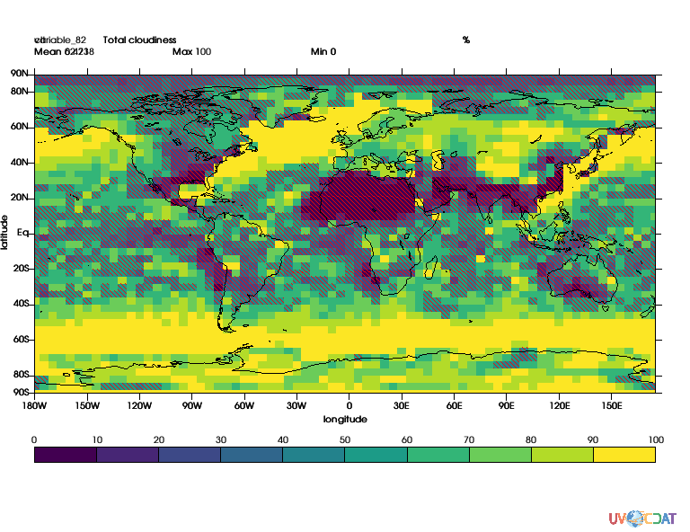
Method 3: Using Patterns
Rather than opacity, we can use patterns, that let us see better what’s “underneath” (top)
[7]:
gm2.fillareastyle = "pattern"
gm2.fillareaindices = [10]
gm2.fillareaopacity = [100]
x.clear()
x.plot(clt,gm)
x.plot(bad,gm2,tmpl2)
[7]:

[8]:
# we can control the size of patterns
gm2.fillareapixelscale = 2.
x.clear()
x.plot(clt,gm)
x.plot(bad,gm2,tmpl2)
[8]:

Controling Patterns Size
We can make the patterns bigger or smaller, using spacing (top)
[9]:
# Bigger
gm2.fillareapixelspacing = [20,20]
gm2.fillareapixelscale=None
x.clear()
x.plot(clt,gm)
x.plot(bad,gm2,tmpl2)
[9]:
[10]:
# or smaller
gm2.fillareapixelspacing = [5,5]
gm2.fillareapixelscale=None
x.clear()
x.plot(clt,gm)
x.plot(bad,gm2,tmpl2)
[10]:
Size and Opacity
We can still add opacity (top)
[11]:
gm2.fillareaopacity = [25.]
x.clear()
x.plot(clt,gm)
x.plot(bad,gm2,tmpl2)
[11]: